The Bellman equation of optimality

To explain the Bellman equation, it's better to go a bit abstract. Don't be afraid, I'll provide the concrete examples later to support your intuition! Let's start with a deterministic case, when all our actions have a 100% guaranteed outcome. Imagine that our agent observes state and has N available actions. Every action leads to another state, , with a respective reward, . Also assume that we know the values, , of all states connected to the state . What will be the best course of action that the agent can take in such a state?

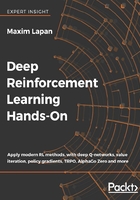
Figure 3: An abstract environment with N states reachable from the initial state

If we choose the concrete action , and calculate the value given to this action, then the value will be . So, to choose the best possible action, the agent needs to calculate the resulting values for every action and choose the maximum possible outcome. In other words: . If we're using discount factor , we need to multiply the value of the next state by gamma: .

This may look very similar to our greedy example from the previous section, and, in fact, it is. However, there is one difference: when we act greedily, we do not only look at the immediate reward for the action, but at the immediate reward plus the long-term value of the state. Richard Bellman proved that with that extension, our behavior will get the best possible outcome. In other words, it will be optimal. So, the preceding equation is called the Bellman equation of value (for a deterministic case):

It's not very complicated to extend this idea for a stochastic case, when our actions have the chance to end up in different states. What we need to do is to calculate the expected value for every action, instead of just taking the value of the next state. To illustrate this, let's consider one single action available from state , with three possible outcomes.

Figure 4: An example of the transition from the state in a stochastic case

Here we have one action, which can lead to three different states with different probabilities: with probability it can end up in state , in state , and in state (, of course). Every target state has its own reward (,, or ). To calculate the expected value after issuing action 1, we need to sum all values, multiplied by their probabilities:

or more formally,

By combining the Bellman equation, for a deterministic case, with a value for stochastic actions, we get the Bellman optimality equation for a general case:

(Note that means the probability of action a, issued in state i, to end up in state j.)

The interpretation is still the same: the optimal value of the state is equal to the action, which gives us the maximum possible expected immediate reward, plus discounted long-term reward for the next state. You may also notice that this definition is recursive: the value of the state is defined via the values of immediate reachable states.

This recursion may look like cheating: we define some value, pretending that we already know it. However, this is a very powerful and common technique in computer science and even in math in general (proof by induction is based on the same trick). This Bellman equation is a foundation not only in RL but also in much more general dynamic programming, which is a widely used method for solving practical optimization problems.

These values not only give us the best reward that we can obtain, but they basically give us the optimal policy to obtain that reward: if our agent knows the value for every state, then it automatically knows how to gather all this reward. Thanks to Bellman's optimality proof, at every state the agent ends up in, it needs to select the action with the maximum expected reward for the action, which is a sum of the immediate reward and the one-step discounted long-term reward. That's it. So, those values are really useful stuff to know. Before we get familiar with a practical way to calculate them, we need to introduce one more mathematical notation. It's not as fundamental as value, but we need it for our convenience.