Example – GAN on Atari images

Almost every book about DL uses the MNIST dataset to show you the power of DL, which, over the years, has made this dataset extremely boring, like a fruit fly for genetic researchers. To break this tradition, and add a bit more fun to the book, I've tried to avoid well-beaten paths and illustrate PyTorch using something different. You may have heard about generative adversarial networks (GANs), which were invented and popularized by Ian Goodfellow. In this example, we'll train a GAN to generate screenshots of various Atari games.

The simplest GAN architecture is this: we have two networks and the first works as a "cheater" (it is also called generator), and the other is a "detective" (another name is discriminator). Both networks compete with each other: the generator tries to generate fake data, which will be hard for the discriminator to distinguish from your dataset, and the discriminator tries to detect the generated data samples. Over time, both networks improve their skills: the generator produces more and more realistic data samples, and the discriminator invents more sophisticated ways to distinguish the fake items. Practical usage of GANs includes image quality improvement, realistic image generation, and feature learning. In our example, practical usefulness is almost zero, but it will be a good example of how clean and short PyTorch code can be for quite complex models.

So, let's get started. The whole example code is in the file Chapter03/03_atari_gan.py. Here we'll look at only significant pieces of code, without the import section and constants declaration:

class InputWrapper(gym.ObservationWrapper):
    def __init__(self, *args):
        super(InputWrapper, self).__init__(*args)
        assert isinstance(self.observation_space, gym.spaces.Box)
        old_space = self.observation_space
        self.observation_space = gym.spaces.Box(self.observation(old_space.low),self.observation(old_space.high), dtype=np.float32)

    def observation(self, observation):
        # resize image
        new_obs = cv2.resize(observation, (IMAGE_SIZE, IMAGE_SIZE))
        # transform (210, 160, 3) -> (3, 210, 160)
        new_obs = np.moveaxis(new_obs, 2, 0)
        return new_obs.astype(np.float32) / 255.0

This class is a wrapper around a Gym game, which includes several transformations:

• Resize input image from 210 × 160 (standard Atari resolution) to a square size 64 × 64
• Move color plane of the image from the last position to the first, to meet the PyTorch convention of convolution layers that input a tensor with the shape of channels, height, and width
• Cast the image from bytes to float and rescale its values to a 0..1 range

Then we define two nn.Module classes: Discriminator and Generator. The first takes our scaled color image as input and, by applying five layers of convolutions, converts it into a single number, passed through a sigmoid nonlinearity. The output from Sigmoid is interpreted as the probability that Discriminator thinks our input image is from the real dataset.

Generator takes as input a vector of random numbers (latent vector) and using the "transposed convolution" operation (it is also known as deconvolution), converts this vector into a color image of the original resolution. We will not look at those classes here as they are lengthy and not very relevant to our example. You can find them in the complete example file.

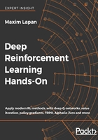
Figure 6: A sample screenshot from three Atari games

As input, we'll use screenshots from several Atari games played simultaneously by a random agent. Figure 6 is an example of what the input data looks like and it is generated by the following function:

def iterate_batches(envs, batch_size=BATCH_SIZE):
    batch = [e.reset() for e in envs]
    env_gen = iter(lambda: random.choice(envs), None)

    while True:
        e = next(env_gen)
        obs, reward, is_done, _ = e.step(e.action_space.sample())
        if np.mean(obs) > 0.01:
            batch.append(obs)
        if len(batch) == batch_size:
            yield torch.FloatTensor(batch)
            batch.clear()
        if is_done:
            e.reset()

This infinitely samples the environment from the provided array, issues random actions and remembers observations in the batch list. When the batch becomes of the required size, we convert it to a tensor and yield from the generator. The check for the nonzero mean of the observation is required due to a bug in one of the games to prevent the flickering of an image.

Now let's look at our main function, which prepares models and runs the training loop:

if __name__ == "__main__":
    parser = argparse.ArgumentParser()
    parser.add_argument("--cuda", default=False, action='store_true')
    args = parser.parse_args()
    device = torch.device("cuda" if args.cuda else "cpu")

    env_names = ('Breakout-v0', 'AirRaid-v0', 'Pong-v0')
    envs = [InputWrapper(gym.make(name)) for name in env_names]
    input_shape = envs[0].observation_space.shape

Here, we process the command-line arguments (which could be only one optional argument, --cuda, enabling GPU computation mode) and create our environment pool with a wrapper applied. This environment array will be passed to the iterate_batches function to generate training data:

    Writer = SummaryWriter()
    net_discr = Discriminator(input_shape=input_shape).to(device)
    net_gener = Generator(output_shape=input_shape).to(device)

    objective = nn.BCELoss()
    gen_optimizer = optim.Adam(params=net_gener.parameters(), lr=LEARNING_RATE)
    dis_optimizer = optim.Adam(params=net_discr.parameters(), lr=LEARNING_RATE)

In this piece, we create our classes: a summary writer, both networks, a loss function, and two optimizers. Why two? It's because that's the way that GANs get trained: to train the discriminator, we need to show it both real and fake data samples with appropriate labels (1 for real, 0 for fake). During this pass, we update only the discriminator's parameters.

After that, we pass both real and fake samples through the discriminator again, but this time the labels are 1s for all samples, and now we update only the generator's weights. The second pass teaches the generator how to fool the discriminator and confuse real samples with the generated ones:

    gen_losses = []
    dis_losses = []
    iter_no = 0

    true_labels_v = torch.ones(BATCH_SIZE, dtype=torch.float32, device=device)
    fake_labels_v = torch.zeros(BATCH_SIZE, dtype=torch.float32, device=device)

Here, we define arrays, which will be used to accumulate losses, iterator counters, and variables with the True and Fake labels.

    for batch_v in iterate_batches(envs):
        # generate extra fake samples, input is 4D: batch, filters, x, y
        gen_input_v = torch.FloatTensor(BATCH_SIZE, LATENT_VECTOR_SIZE, 1, 1).normal_(0, 1).to(device)
        batch_v = batch_v.to(device)
        gen_output_v = net_gener(gen_input_v)

At the beginning of the training loop, we generate a random vector and pass it to the Generator network.

        dis_optimizer.zero_grad()
        dis_output_true_v = net_discr(batch_v)
        dis_output_fake_v = net_discr(gen_output_v.detach())
        dis_loss = objective(dis_output_true_v, true_labels_v) + objective(dis_output_fake_v, fake_labels_v)
        dis_loss.backward()
        dis_optimizer.step()
        dis_losses.append(dis_loss.item())

At first, we train the discriminator by applying it two times: to the true data samples in our batch and to the generated ones. We need to call the detach() function on the generator's output to prevent gradients of this training pass from flowing into the generator (detach() is a method of tensor, which makes a copy of it without connection to the parent's operation).

        gen_optimizer.zero_grad()
        dis_output_v = net_discr(gen_output_v)
        gen_loss_v = objective(dis_output_v, true_labels_v)
        gen_loss_v.backward()
        gen_optimizer.step()
        gen_losses.append(gen_loss_v.item())

Now it's the generator's training time. We pass the generator's output to the discriminator, but now we don't stop the gradients. Instead, we apply the objective function with True labels. It will push our generator in the direction where the samples that it generates make the discriminator confuse them with the real data.

That's all real training, and the next couple of lines report losses and feed image samples to TensorBoard:

        iter_no += 1
        if iter_no % REPORT_EVERY_ITER == 0:
            log.info("Iter %d: gen_loss=%.3e, dis_loss=%.3e",iter_no, np.mean(gen_losses), np.mean(dis_losses))
            writer.add_scalar("gen_loss", np.mean(gen_losses), iter_no)
            writer.add_scalar("dis_loss", np.mean(dis_losses), iter_no)
            gen_losses = []
            dis_losses = []
        if iter_no % SAVE_IMAGE_EVERY_ITER == 0:
            writer.add_image("fake", vutils.make_grid(gen_output_v.data[:64]), iter_no)
            writer.add_image("real", vutils.make_grid(batch_v.data[:64]), iter_no)

The training of this example is quite a lengthy process. On a GTX 1080 GPU, 100 iterations take about 40 seconds. At the beginning, the generated images are completely random noise, but after 10k-20k iterations, the generator becomes more and more proficient at its job and the generated images become more and more similar to the real game screenshots.

My experiments gave the following images after 40k-50k of training iterations (several hours on a GPU):

Figure 7: Sample images produced by the generator network