Designing the warming and cooling effect

With the mechanism to quickly apply a generic curve filter to any image channel in place, we can now turn to the question of how to manipulate the perceived color temperature of an image. Again, the final code will have its own function in the tools module.

If you have a minute to spare, I advise you to play around with the different curve settings for a while. You can choose any number of anchor points and apply the curve filter to any image channel you can think of (red, green, blue, hue, saturation, brightness, lightness, and so on). You could even combine multiple channels, or decrease one and shift another to the desired region. What will the result look like?

However, if the number of possibilities dazzles you, take a more conservative approach. First, by making use of our spline_to_lookup_table function developed in the preceding steps, let's define two generic curve filters: one that (by trend) increases all the pixel values of a channel and one that generally decreases them:

INCREASE_LOOKUP_TABLE = spline_to_lookup_table([0, 64, 128, 192, 256],
                                               [0, 70, 140, 210, 256])
DECREASE_LOOKUP_TABLE = spline_to_lookup_table([0, 64, 128, 192, 256],
                                               [0, 30, 80, 120, 192])

Now, let's examine how we could apply lookup tables to an RGB image. OpenCV has a nice function called cv2.LUT that takes a lookup table and applies it to a matrix. So, first, we have to decompose the image into different channels:

    c_r, c_g, c_b = cv2.split(rgb_image)

Then, we apply a filter to each channel if desired:

    if green_filter is not None:
        c_g = cv2.LUT(c_g, green_filter).astype(np.uint8)

Doing this for all the three channels in an RGB image, we get the following helper function:

def apply_rgb_filters(rgb_image, *,
                      red_filter=None, green_filter=None, blue_filter=None):
    c_r, c_g, c_b = cv2.split(rgb_image)
    if red_filter is not None:
        c_r = cv2.LUT(c_r, red_filter).astype(np.uint8)
    if green_filter is not None:
        c_g = cv2.LUT(c_g, green_filter).astype(np.uint8)
    if blue_filter is not None:
        c_b = cv2.LUT(c_b, blue_filter).astype(np.uint8)
    return cv2.merge((c_r, c_g, c_b))

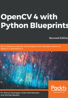
The easiest way to make an image appear as if it was taken on a hot, sunny day (maybe close to sunset) is to increase the reds in the image and make the colors appear vivid by increasing the color saturation. We will achieve this in two steps:

1. Increase the pixel values in the R channel (from RGB image) and decrease the pixel values in the B channel of an RGB color image using INCREASE_LOOKUP_TABLE and DECREASE_LOOKUP_TABLE, respectively:

        interim_img = apply_rgb_filters(rgb_image,
                                        red_filter=INCREASE_LOOKUP_TABLE,
                                        blue_filter=DECREASE_LOOKUP_TABLE)

2. Transform the image into the HSV color space (H means hue, S means saturation, and V means value), and increase the S channel using INCREASE_LOOKUP_TABLE. This can be achieved with the following function, which expects an RGB color image and a lookup table to apply (similar to the apply_rgb_filters function) as input:

def apply_hue_filter(rgb_image, hue_filter):
    c_h, c_s, c_v = cv2.split(cv2.cvtColor(rgb_image, cv2.COLOR_RGB2HSV))
    c_s = cv2.LUT(c_s, hue_filter).astype(np.uint8)
    return cv2.cvtColor(cv2.merge((c_h, c_s, c_v)), cv2.COLOR_HSV2RGB)

The result looks like this:

Analogously, we can define a cooling filter that increases the pixel values in the B channel, decreases the pixel values in the R channel of an RGB image, converts the image into the HSV color space, and decreases color saturation via the S channel:

    def _render_cool(rgb_image: np.ndarray) -> np.ndarray:
        interim_img = apply_rgb_filters(rgb_image,
                                        red_filter=DECREASE_LOOKUP_TABLE,
                                        blue_filter=INCREASE_LOOKUP_TABLE)
        return apply_hue_filter(interim_img, DECREASE_LOOKUP_TABLE)

Now the result looks like this:

Let's explore how to cartoonize an image in the next section, where we'll learn what a bilateral filter is and much more.